Használati útmutató Ibm SPSS 20
Ibm
Irodai szoftverek
SPSS 20
Olvassa el alább 📖 a magyar nyelvű használati útmutatót Ibm SPSS 20 (170 oldal) a Irodai szoftverek kategóriában. Ezt az útmutatót 8 ember találta hasznosnak és 2 felhasználó értékelte átlagosan 4.5 csillagra
Oldal 1/170

i
IBM SPSS Statistics 20 Brief Guide

Note: Before using this information and the product it supports, read the general information
under Notices on p. 156.
This edition applies to IBM® SPSS® Statistics 20 and to all subsequent releases and modifications
until otherwise indicated in new editions.
Adobe product screenshot(s) reprinted with permission from Adobe Systems Incorporated.
Microsoft product screenshot(s) reprinted with permission from Microsoft Corporation.
Licensed Materials - Property of IBM
© C opyright IBM Corporation 1989, 2011.
U.S. Government Users Restricted Rights - Use, duplication or disclosure restricted by GSA ADP
Schedule Contract with IBM Corp.

Preface
The IBM SPSS Statistics 20 Brief Guide provides a set of tutorials designed to acquaint you
with the various components of IBM® SPSS® Statistics. This guide is intended for use with all
operating system versions of the software, including: Windows, Macintosh, and Linux. You
can work through the tutorials in sequence or turn to the topics for which you need additional
information. You can use this guide as a supplement to the online tutorial that is included with the
SPSS Statistics Core system or ignore the online tutorial and start with the tutorials found here.
IBM SPSS Statistics 20
IBM® SPSS® Statistics 20 is a comprehensive system for analyzing data. SPSS Statistics can
take data from almost any type of file and use them to generate tabulated reports, charts, and plots
of distributions and trends, descriptive statistics, and complex statistical analyses.
SPSS Statistics makes statistical analysis more accessible for the beginner and more convenient
for the experienced user. Simple menus and dialog box selections make it possible to perform
complex analyses without typing a single line of command syntax. The Data Editor offers a
simple and efficient spreadsheet-like facility for entering data and browsing the working data file.
Internet Resources
The IBM Corp. Web site (http://www.ibm.com/support) offers answers to frequently asked
questions and provides access to data files and other useful information.
In addition, the SPSS USENET discussion group (not sponsored by IBM Corp.) is open to
anyone interested . The USENET address is comp.soft-sys.stat.spss.
You can also subscribe to an e-mail message list that is gatewayed to the USENET group. To
subscribe, send an e-mail message to listserv@listserv.uga.edu. The text of the e-mail message
should be: subscribe SPSSX-L firstname lastname. You can then post messages to the list by
sending an e-mail message to listserv@listserv.uga.edu.
Additional Publications
The IBM SPSS Statistics Statistical Procedures Companion, by Marija Norušis, has been
published by Prentice Hall. It contains overviews of the procedures in IBM® SPSS® Statistics
Base, plus Logistic Regression and General Linear Models. The IBM SPSS Statistics Advanced
Statistical Procedures Companion has also been published by Prentice Hall. It includes overviews
of the procedures in the Advanced and Regression modules.
IBM SPSS Statistics Options
The following options are available as add-on enhancements to the full (not Student Version)
IBM® SPSS® Statistics system:
Statistics Base gives you a wide range of statistical procedures for basic analyses and reports,
including counts, crosstabs and descriptive statistics, OLAP Cubes and codebook reports. It also
provides a wide variety of dimension reduction, classification and segmentation techniques such
as factor analysis, cluster analysis, nearest neighbor analysis and discriminant function analysis.
© Copyright IBM Corporation 1989, 2011. iii

Additionally, SPSS Statistics Base offers a broad range of algor ing means andithms for compar
predictive techniques such as t-test, analysis of variance, linear regression and ordinal regression.
Advanced Statistics focuses on techniques often used in sophisticated experimental and biomedical
research. It includes procedures for general linear models (GLM), linear mixed models, variance
components analysis, loglinear analysis, ordinal regression, actuarial life tables, Kaplan-Meier
survival analysis, and basic and extended Cox regression.
Bootstrapping is a method for deriving robust estimates of standard errors and confidence
intervals for estimates such as the mean, median, proportion, odds ratio, correlation coefficient or
regression coefficient.
Categories performs optimal scaling procedures, including correspondence analysis.
Complex Samples allows survey, market, health, and public opinion researchers, as well as social
scientists who use sample survey methodology, to incorporate their complex sample designs
into data analysis.
Conjoint provides a realistic way to measure how individual product attributes affect consumer and
citizen preferences. With Conjoint, you can easily measure the trade-off effect of each product
attribute in the context of a set of product attributes—as consumers do when making purchasing
decisions.
Custom Tables creates a variety of presentation-quality tabular reports, including complex
stub-and-banner tables and displays of multiple response data.
Data Preparation provides a quick visual snapshot of your data. It provides the ability to apply
validation rules that identify invalid data values. You can create rules that flag out-of-range
values, missing values, or blank values. You can also save variables that record individual rule
violations and the total number of rule violations per case. A limited set of predefined rules that
you can copy or modify is provided.
Decision Trees creates a tree-based classification model. It classifies cases into groups or predicts
values of a dependent (target) variable based on values of independent (predictor) variables. The
procedure provides validation tools for exploratory and confirmatory classification analysis.
Direct Marketing allows organizations to ensure their marketing programs are as effective as
possible, through techniques specifically designed for direct marketing.
Exact Tests calculates exact pvalues for statistical tests when small or very unevenly distributed
samples could make the usual tests inaccurate. This option is available only on Windows
operating systems.
Forecasting performs comprehensive forecasting and time series analyses with multiple
curve-fitting models, smoothing models, and methods for estimating autoregressive functions.
Missing Values describes patterns of missing data, estimates means and other statistics, and
imputes values for missing observations.
Neural Networks can be used to make business decisions by forecasting demand for a product as a
function of price and other variables, or by categorizing customers based on buying habits and
demographic characteristics. Neural networks are non-linear data modeling tools. They can be
used to model complex relationships between inputs and outputs or to find patterns in data.
iv

Regression provides techniques for analyzing data that do not fit traditional linear statistical
models. It includes procedures for probit analysis, logistic regression, weight estimation,
two-stage least-squares regression, and general nonlinear regression.
Amos™ (analysis of moment structures) uses structural equation modeling to confirm and explain
conceptual models that involve attitudes, perceptions, and other factors that drive behavior.
Training Seminars
IBM Corp. provides both public and onsite training seminars for IBM® SPSS® Statistics.
All seminars feature hands-on workshops. seminars will be offered in major U.S. and
European cities on a regular basis. For more information on these seminars, go to
http://www.ibm.com/software/analytics/spss/training/.
Technical support
Technical support is available to maint enance customers. Cu stomers may c ontact Techn ical
Support for assistance in using IBM Corp. products or for installation help for one of the
supported hardware environments. To reach Technical Support, see the IBM Corp. web site
at http://www.ibm.com/support. Be prepared to identify yourself, your organization, and your
support a greement when requestin g assi stance.
IBM SPSS Statistics 20 Student Version
The IBM® SPSS® Statistics 2 0 Student Version is a limited but still powerful version of SPSS
Statistics.
Capability
The Student Version contains many of the important data analysis tools contained in IBM®
SPSS® Statistics, including:
Spreadsheet-like Data Editor for entering, modifying, and viewing data files.
Statistical procedures, including ttests, analysis of variance, and crosstabulations.
Interactive graphics that allow you to change or add chart elements and variables dynamically;
the changes appear as soon as they are specified.
Standard high-resolution graphics for an extensive array of analytical and presentation charts
and tables.
Limitations
Created for classroom instruction, the Student Version is limited to use by students and instructors
for educational purposes only. The following limitations apply to the IBM® SPSS® Statistics 20
Student Version:
Data files cannot contain more than 50 variables.
Data files cannot contain more than 1,500 cases. SPSS Statistics add-on modules (such as
Regression or Advanced Statistics) cannot be used with the Student Version.
v

SPSS Statistics command syntax is not available to the user. This means that it is not possible
to repeat an analysis by saving a series of commands in a syntax or “job” file, as can be done
in the full version of IBM® SPSS® Statistics.
Scripting and automation are not available to the user. This means that you cannot create
scripts that automate tasks that you repeat often, as can be done in the full version of SPSS
Statistics.
Technical Support for Students
If you’re a student using a student, academic or grad pack version of any IBM
SPSS software product, please see our special online Solutions for Education
(http://www.ibm.com/spss/rd/students/)pages for students. If you’re a student using a
university-supplied copy of the IBM SPSS software, please contact the IBM SPSS product
coordinator at your university.
Technical Support for Instructors
Instructors using the Student Version for classroom instruction may contact Technical Support for
assistance. In the United States and Canada, call Technical Support at (312) 651-3410, or send
go to http://www.ibm.com/support.
vi

Contents
1 Introduction 1
SampleFiles................................................................. 1
Opening a Data File. . . . . . . . . . . . . . . . . . . . . . . . . . . . . . . . . . . . . . . . . . . . . . . . . . . . . . . . . . . . 1
RunninganAnalysis .......................................................... 3
ViewingResults.............................................................. 6
CreatingCharts............................................................... 7
2 Reading Data 10
Basic Structure of IBM SPSS Statistics Data Files . . . . . . . . . . . . . . . . . . . . . . . . . . . . . . . . . . . . 10
Reading IBM SPSS Statistics Data Files . . . . . . . . . . . . . . . . . . . . . . . . . . . . . . . . . . . . . . . . . . . . 10
Reading Data from Spreadsheets . . . . . . . . . . . . . . . . . . . . . . . . . . . . . . . . . . . . . . . . . . . . . . . . . 11
Reading Data from a Database . . . . . . . . . . . . . . . . . . . . . . . . . . . . . . . . . . . . . . . . . . . . . . . . . . . 12
Reading Data fromaTextFile....................................................18
3 Using the Data Editor 26
Entering Numeric Data . . . . . . . . . . . . . . . . . . . . . . . . . . . . . . . . . . . . . . . . . . . . . . . . . . . . . . . . . 26
Entering String Data . . . . . . . . . . . . . . . . . . . . . . . . . . . . . . . . . . . . . . . . . . . . . . . . . . . . . . . . . . . 28
DefiningData................................................................30
Adding Variable Labels . . . . . . . . . . . . . . . . . . . . . . . . . . . . . . . . . . . . . . . . . . . . . . . . . . . . . 30
Changing Variable Type and Format . . . . . . . . . . . . . . . . . . . . . . . . . . . . . . . . . . . . . . . . . . . . 31
Adding Value Labels for Numeric Variables . . . . . . . . . . . . . . . . . . . . . . . . . . . . . . . . . . . . . . 31
Adding Value Labels for String Variables . . . . . . . . . . . . . . . . . . . . . . . . . . . . . . . . . . . . . . . . 33
Using Value Labels for Data Entry . . . . . . . . . . . . . . . . . . . . . . . . . . . . . . . . . . . . . . . . . . . . . 34
Handling Missing Data. . . . . . . . . . . . . . . . . . . . . . . . . . . . . . . . . . . . . . . . . . . . . . . . . . . . . . 35
Missing Values for a Numeric Variable. . . . . . . . . . . . . . . . . . . . . . . . . . . . . . . . . . . . . . . . . . 36
Missing Values for a String Variable. . . . . . . . . . . . . . . . . . . . . . . . . . . . . . . . . . . . . . . . . . . . 37
Copying and Pasting Variable Attributes . . . . . . . . . . . . . . . . . . . . . . . . . . . . . . . . . . . . . . . . 38
Defining Variable Properties for Categorical Variables . . . . . . . . . . . . . . . . . . . . . . . . . . . . . . 42
4 Working with Multiple Data Sources 49
Basic Handling of Multiple Data Sources . . . . . . . . . . . . . . . . . . . . . . . . . . . . . . . . . . . . . . . . . . . 49
Working with Multiple Datasets in Command Syntax. . . . . . . . . . . . . . . . . . . . . . . . . . . . . . . . . . . 50
vii

Hiding Rows and Columns . . . . . . . . . . . . . . . . . . . . . . . . . . . . . . . . . . . . . . . . . . . . . . . . . . . 89
Changing Data Display Formats . . . . . . . . . . . . . . . . . . . . . . . . . . . . . . . . . . . . . . . . . . . . . . . 89
TableLooks . . . . . . . . . . . . . . . . . . . . . . . . . . . . . . . . . . . . . . . . . . . . . . . . . . . . . . . . . . . . . . . . . . 91
Using Predefined Formats . . . . . . . . . . . . . . . . . . . . . . . . . . . . . . . . . . . . . . . . . . . . . . . . . . . 91
Customizing TableLook Styles . . . . . . . . . . . . . . . . . . . . . . . . . . . . . . . . . . . . . . . . . . . . . . . . 92
Changing the Default Table Formats. . . . . . . . . . . . . . . . . . . . . . . . . . . . . . . . . . . . . . . . . . . . 94
Customizing the Initial Display Settings . . . . . . . . . . . . . . . . . . . . . . . . . . . . . . . . . . . . . . . . . 96
Displaying Variable and Value Labels. . . . . . . . . . . . . . . . . . . . . . . . . . . . . . . . . . . . . . . . . . . 97
Using Results in Other Applications . . . . . . . . . . . . . . . . . . . . . . . . . . . . . . . . . . . . . . . . . . . . . . . 99
Pasting Results as Word Tables . . . . . . . . . . . . . . . . . . . . . . . . . . . . . . . . . . . . . . . . . . . . . . . 99
Pasting Results as Text . . . . . . . . . . . . . . . . . . . . . . . . . . . . . . . . . . . . . . . . . . . . . . . . . . . . 100
Exporting Results to Microsoft Word, PowerPoint, and Excel Files . . . . . . . . . . . . . . . . . . . . 101
Exporting Results to PDF . . . . . . . . . . . . . . . . . . . . . . . . . . . . . . . . . . . . . . . . . . . . . . . . . . . 108
Exporting Results to HTML . . . . . . . . . . . . . . . . . . . . . . . . . . . . . . . . . . . . . . . . . . . . . . . . . . 111
8 Working with Syntax 112
Pasting Syntax . . . . . . . . . . . . . . . . . . . . . . . . . . . . . . . . . . . . . . . . . . . . . . . . . . . . . . . . . . . . . . 112
Editing Syntax. . . . . . . . . . . . . . . . . . . . . . . . . . . . . . . . . . . . . . . . . . . . . . . . . . . . . . . . . . . . . . . 113
Opening and Running a Syntax File . . . . . . . . . . . . . . . . . . . . . . . . . . . . . . . . . . . . . . . . . . . . . . . 115
Understanding the Error Pane. . . . . . . . . . . . . . . . . . . . . . . . . . . . . . . . . . . . . . . . . . . . . . . . . . . 116
Using Breakpoints . . . . . . . . . . . . . . . . . . . . . . . . . . . . . . . . . . . . . . . . . . . . . . . . . . . . . . . . . . . 116
9 Modifying Data Values 119
Creating a Categorical Variable from a Scale Variable. . . . . . . . . . . . . . . . . . . . . . . . . . . . . . . . . 119
Computing New Variables. . . . . . . . . . . . . . . . . . . . . . . . . . . . . . . . . . . . . . . . . . . . . . . . . . . . . . 125
Using Functions in Expressions . . . . . . . . . . . . . . . . . . . . . . . . . . . . . . . . . . . . . . . . . . . . . . 127
Using Conditional Expressions . . . . . . . . . . . . . . . . . . . . . . . . . . . . . . . . . . . . . . . . . . . . . . . 129
Working with Dates and Times . . . . . . . . . . . . . . . . . . . . . . . . . . . . . . . . . . . . . . . . . . . . . . . . . . 131
Calculating the Length of Time between Two Dates . . . . . . . . . . . . . . . . . . . . . . . . . . . . . . . 132
Adding a Duration to a Date . . . . . . . . . . . . . . . . . . . . . . . . . . . . . . . . . . . . . . . . . . . . . . . . . 135
10 Sorting and Selecting Data 138
Sorting Data . . . . . . . . . . . . . . . . . . . . . . . . . . . . . . . . . . . . . . . . . . . . . . . . . . . . . . . . . . . . . . . . 138
ix

Chapter
Introduction
This guide provides a set of tutorials designed to enable you to perform useful analyses on your
data. You can work through the tutorials in sequence or turn to the topics for which you need
additional information.
This chapter will introduce you to the basic features and demonstrate a typical session. We
will retrieve a previously defined IBM® SPSS® Statistics data file and then produce a simple
statistical summary and a chart.
More detailed instruction about many of the topics touched upon in this chapter will follow in
later chapters. Here, we hope to give you a basic framework for understanding later tutorials.
Sample Files
Most of the examples that are presented here use the data file demo.sav. This data file is a fictitious
survey of several thousand people, containing basic demographic and consumer information.
If you are using the Student version, your version of demo.sav is a representative sample of the
original data file, reduced to meet the 1,500-case limit. Results that you obtain using that data
file will differ from the results shown here.
The sample files installed with the product can be found in the Samples subdirectory of the
installation directory. There is a separate folder within the Samples subdirectory for each of
the following languages: English, French, German, Italian, Japanese, Korean, Polish, R ussian,
Simplified Chinese, Spanish, and Traditional Chinese.
Not all sample files are available in all languages. If a sample file is not available in a language,
that language folder contains an English version of the sample file.
Opening a Data File
To open a data file:
EFrom the menus choose:
File > Open > D ata...
Alternatively, you can use the Open File button on the toolbar.
Figure 1-1
Open File to olbar button
A dialog box for opening files is displayed.
© Copyright IBM Corporation 1989, 2011. 1
2
Chapter 1
By default, IBM® SPSS® Statistics data files (.sav extension) are displayed.
This example uses the file demo.sav.
Figure 1-2
demo.sav file in Data Editor
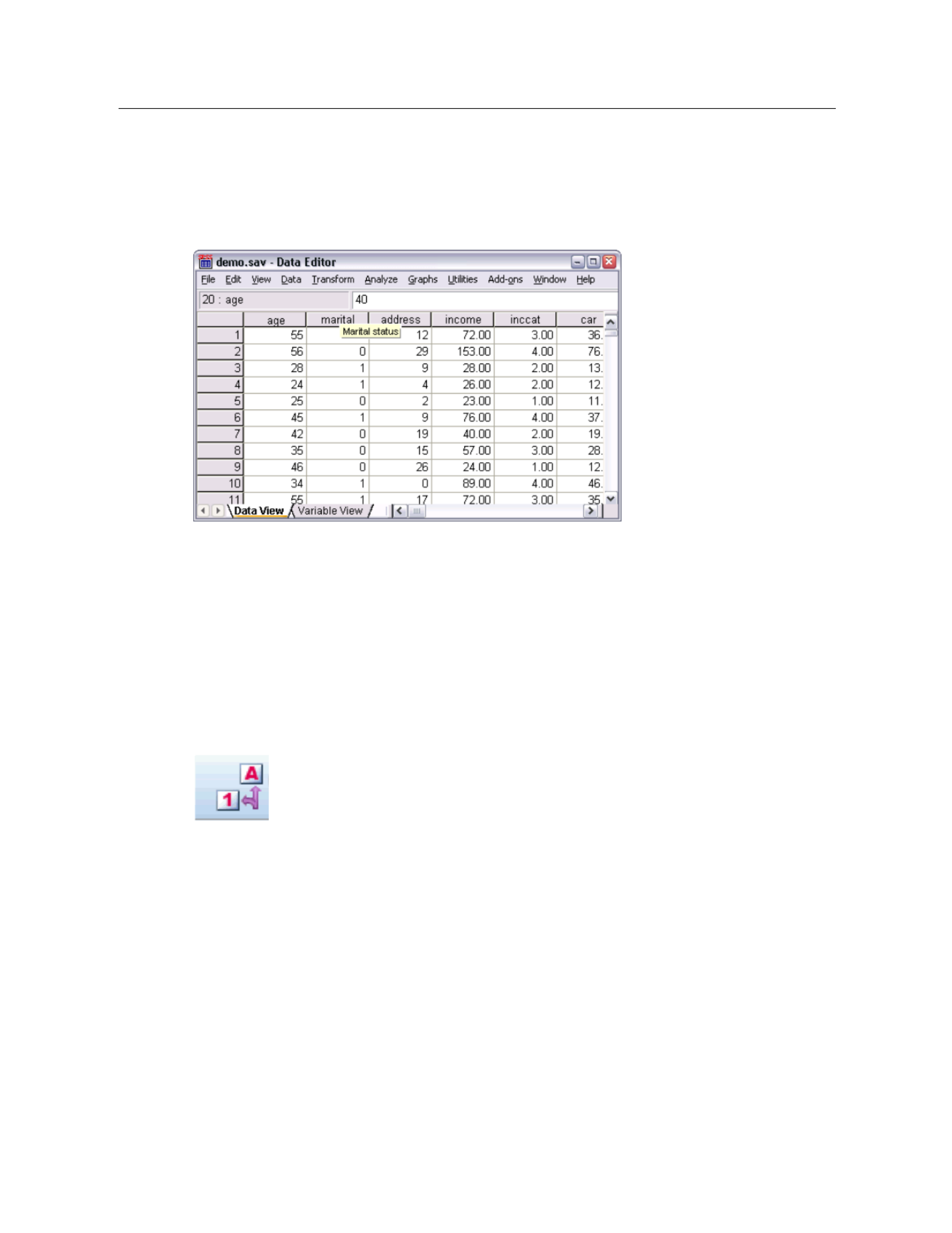
The data file is displayed in the D ata Editor. In the Data Editor, if you put the mouse cursor on a
variable name (the column headings), a more descriptive variable label is displayed (if a label
has been defined for that variable).
By default, the actual data v alues are displayed. To display labels:
EFrom the menus choose:
View > Value Labels
Alternatively, you can use the Value Labels button on the toolbar.
Figure 1-3
Value Labels button
Descriptive value labels are now displayed to make it easier to interpret the responses.

3
Introduction
Figure 1-4
Value labels displayed in the Data Editor
Running an Analysis
If you have any add-on options, the Analyze menu contains a list of reporting and statistical
analysis categories.
We will start by creating a simple frequency table (table of counts). This example requires the
Statistics Base option.
EFrom the menus choose:
Analyze > Descriptive Statistics > Frequencies...
The Frequencies dialog box is displayed.
Figure 1-5
Frequencies dialo g box

4
Chapter 1
An icon next to each variable provides information about data type and level of measurement.
Numeric String Date Time
Scale (Continuous) n/a
Ordinal
Nominal
EClick the variable Income category in thousands [inccat].
Figure 1-6
Variable labels and names in the Frequencies dialog box
If the variable label and/or name appears truncated in the list, the complete label/name is displayed
when the cursor is positioned over it. The variable name inccat is displayed in square brackets
after the descriptive variable label. Income category in thousands is the variable label. If there
were no variable label, only the variable name would appear in the list box.
You can resize dialog boxes just like windows, by clicking and dragging the outside borders or
corners. For example, if you make the dialog box wider, the variable lists will also be wider.

5
Introduction
Figure 1-7
Resized dialog box
In the dialog box, you choose the variables that you want to analyze from the source list on the
left and drag and drop them into the Variable(s) list on the right. The OK button, which runs the
analysis, is disabled until at least one variable is placed in the Variable(s) list.
In many dialogs, you can obtain additional information by right-clicking any variable name
in the list.
ERight-click Income category in thousands [inccat] and choose Variable Information.
EClick the down arrow on the Value labels drop-down list.
Figure 1-8
Defined labels for income variable
All of the defined value labels for the variable are displayed.

6
Chapter 1
EClick Gender [gender] in the source variable list and drag the variable into the target Variable(s)
list.
EClick Income category in thousands [inccat] in the source list and drag it to the target list.
Figure 1-9
Variables s elec ted for analysi s
EClick OK to run the procedure.
Viewing Results
Figure 1-10
Viewer window
Results are displayed in the Viewer window.
You can quickly go to any item in the Viewer by selecting it in the outline pane.

7
Introduction
EClick Income category in thousand s [inccat].
Figure 1-11
Frequency table of income categories
The frequency table for income categories is displayed. This frequency table shows the number
and percentage of people in each income category.
Creating Charts
Although some statistical procedures can create charts, you can also use the Graphs menu to
create charts.
For example, you can create a chart that shows the relationship between wireless telephone
service and PDA (personal digital assistant) ownership.
EFrom the menus choose:
Graphs > Chart Builder...
EClick the Gallery tab (if it is not selected).
EClick Bar (if it is not selected).
EDrag the Clustered Bar icon onto the canvas, which is the large area above the Gallery.

8
Chapter 1
Figure 1-12
Chart Builder dialog box
EScroll down the Variables list, right-click Wireless service [wireless], and then choose Nominal
as its measurement level.
EDrag the Wireless service [wireless] variable to the xaxis.
ERight-click Owns PDA [ownpda] and choose Nominal as its measurement level.
EDrag the Owns PDA [ownpda] variable to the cluster drop zone in the upper right corner of
the canvas.
EClick OK to create the chart.

9
Introduction
Figure 1-13
Bar chart displayed in Viewer window
The bar chart is displayed in the Viewer. The chart shows that people with wireless phone service
are far more likely to have PDAs than people without wireless service.
You can edit charts and tables by double-clicking them in the contents pane of the Viewer
window, and you can copy and paste your results into other applications. Those topics will be
covered later.

Chapter
Reading Data
Data can be entered directly, or it can be imported from a number of different sources. The
processes for reading data stored in IBM® SPSS® Statistics data files; spreadsheet applications,
such as Microsoft Excel; database applications, such as Microsoft Access; and text files are
all discussed in this c hapter.
Basic Structure of IBM SPSS Statistics Data Files
Figure 2-1
Data Editor
IBM® SPSS® Statistics data files are organized by cases (rows) and variables (columns). In this
data file, cases represent individual respondents to a survey. Variab les r epresent responses to
each question asked in the survey.
Reading IBM SPSS Statistics Data Files
IBM® SPSS® Statistics data files, which have a .sav file extension, contain your saved data. To
open demo.sav, an example file installed with the product:
EFrom the menus choose:
File > Open > Data...
EBrowse to and open demo.sav.For more information, see the topic Sample Files in Appendix A
on p. 147.
© Copyright IBM Corporation 1989, 2011. 10

11
Reading Data
The data are now displayed in the Data Editor.
Figure 2-2
Opened data file
Reading Data from Spreadsheets
Rather than typing all of your data directly into the Data Editor, you can read data from
applications such as Microsoft Excel. You can also read column headings as variable names.
EFrom the menus choose:
File > Open > Data...
ESelect Excel (*.xls) as the file type you want to view.
EOpen demo.xls.For more information, see the topic Sample Files in Appendix A on p. 147.
The Opening Excel Data Source dialog box is displayed, allowing you to specify whether variable
names are to be included in the spreadsheet, as well as the cells that you want to import. In Excel
95 or later, you can also specify which worksheets you want to import.
Figure 2-3
Opening Excel Data Source dialog box

12
Chapter 2
EMake sure that Read variable names from the first row of data is selected. This option reads column
headings as variable names.
If the column headings do not conform to the IBM® SPSS® Statistics variable-naming rules, they
are converted into valid variable names and the original column headings are saved as variable
labels. If you want to import only a portion of the spreadsheet, specify the range of cells to
be imported in the Range text box.
EClick OK to read the Excel file.
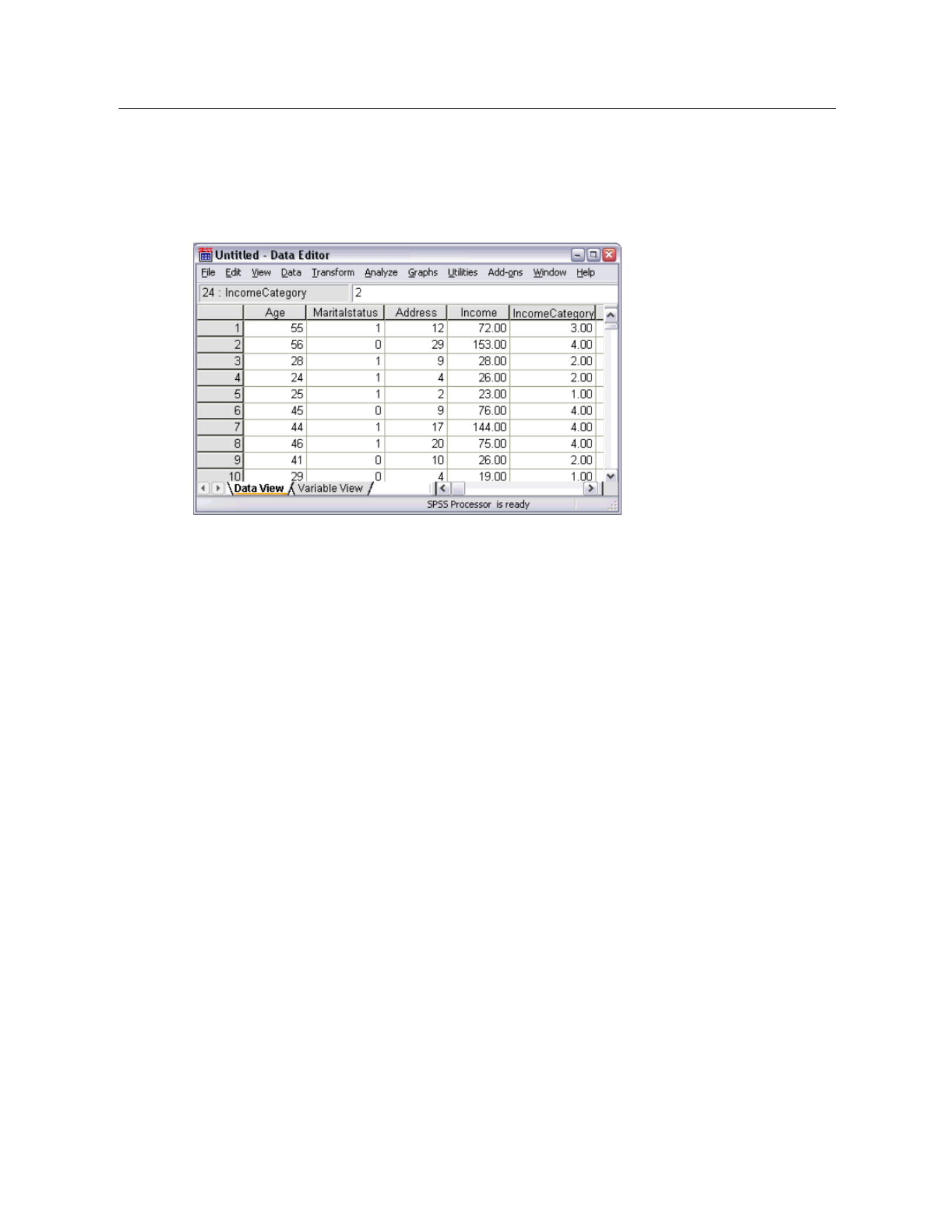
The data now appear in the Data Editor, with the column headings used as variable names. Since
variable names can’t contain spaces, the spaces from the original column headings have been
removed. For example, Marital status in the Excel file becomes the variable Maritalstatus. The
original column heading is retained as a variable label.
Figure 2-4
Imported Excel data
Reading Data from a Database
Data from database sources are easily imported using the Database Wizard. Any database that uses
ODBC (Open Database Connectivity) drivers can be read directly after the drivers are installed.
ODBC drivers for many database formats are supplied on the installation CD. Additional drivers
can be obtained from third-party vendors. One of the most common database applications,
Microsoft Access, is discussed in this example.
Note: This example is specific to Microsoft Windows and requires an ODBC driver for Access.
The steps are similar on other platforms b ut may require a third-party ODBC driver for Access.
EFrom the menus choose:
File > Open Database > New Quer y...

13
Reading Data
Figure 2-5
Dat a base Wizard Welcome dialog box
ESelect MS Access Database from the list of data sources and click Next.
Note: Depending on your installation, you may also see a list of OLEDB data sources on the left
side of the wizard (Windows operating systems only), but this example uses the list of ODBC data
sources displayed on the right side.

14
Chapter 2
Figure 2-6
ODBC Driver Login dialog box
EClick Browse to navigate to the Access database file that you w ant to open.
EOpen demo.mdb.For more information, see the topic Sample Files in Appendix A on p. 147.
EClick OK in the login dialog box.
In the n ext step, you can specify the tables and variables that you w ant to import.
Figure 2-7
Select Dat a step

15
Reading Data
EDrag the entire demo table to the Retrieve Fields In This Order list.
EClick Next.
In the next step, you select which records (cases) to import.
Figure 2-8
Limit Retrieved Cases step
If you do not want t o i mport all cases, y ou can imp ort a subset of cases (for example, males
older than 30), or you can import a random sample of cases from the data source. For large data
sources, you may want to limit the number of cases to a small, representative sample to reduce
the processing time.
EClick Next to continue.
18
Chapter 2
All of the data in the Access database that you selected to import are now available in the Data
Editor.
Figure 2-11
Data imported from an Access database
Reading Data from a Text File
Text files are another common source of data. Many spreadsheet programs and databases can save
their contents in one of many text file formats. Comma- or tab-delimited files refer to rows of data
that use commas or tabs to indicate each variable. In this example, the data are tab delimited.
EFrom the menus choose:
File > Read Text Data...
ESelect Text (*.txt) as the file type you want to view.
EOpen demo.txt.For more information, see the topic Sample Files in Appendix A on p. 147.

19
Reading Data
The Text Import Wizard guides you through the process of defining how the specified text file
should be interpreted.
Figure 2-12
Text Import Wizard: Step 1 of 6
EIn Step 1, you can choose a predefined format or create a new format in the wizard. Select No to
indicate that a new format should be created.
EClick Next to continue.
20
Chapter 2
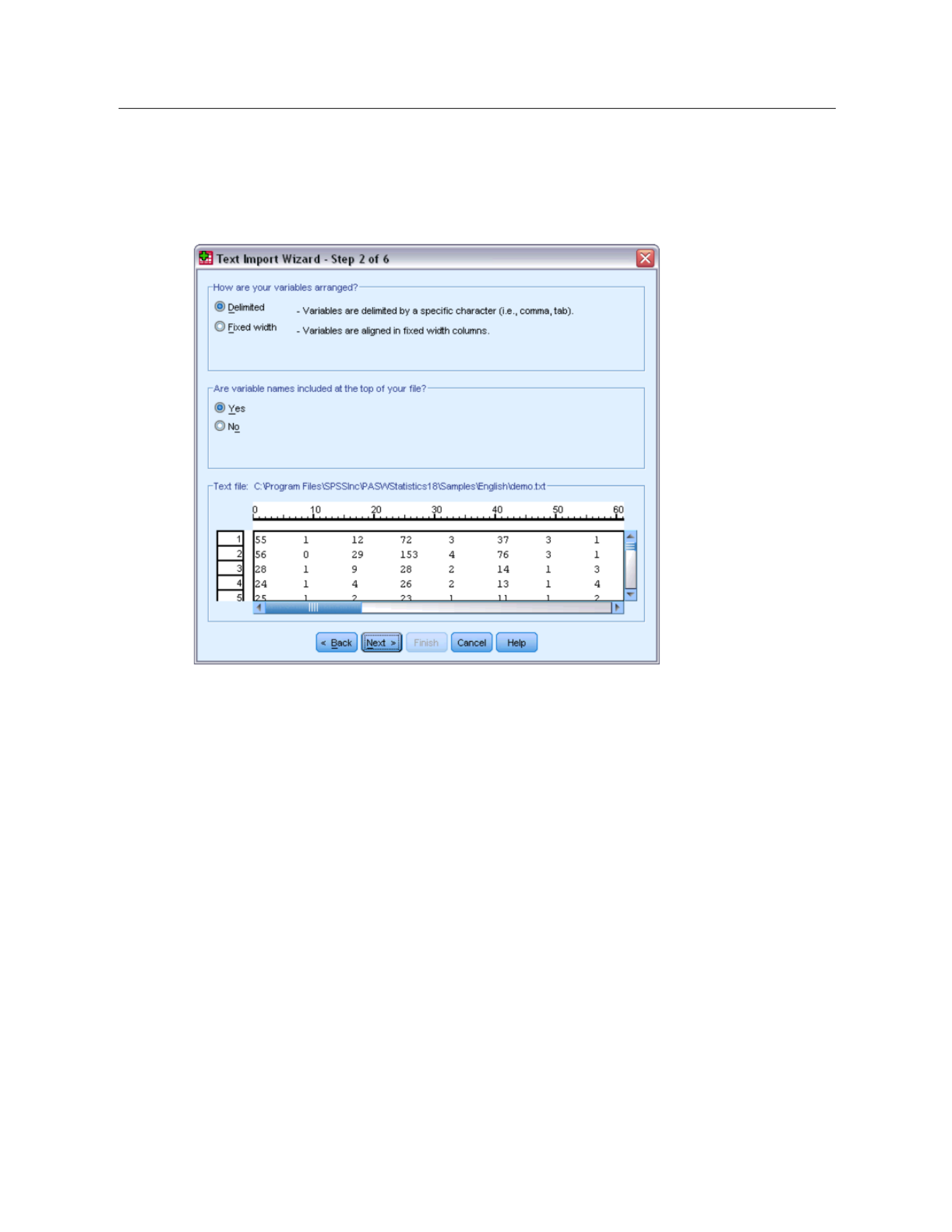
As stated earlier, this file uses tab-delimited formatting. Also, the variable names are defined
on the top line of this file.
Figure 2-13
Text Import Wizard: Step 2 of 6
ESelect Delimited to indicate that the data use a d elimited formatting structure.
ESelect Yes to indicate that variable names should be read from the top of the file.
EClick Next to continue.

21
Reading Data
EType 2in the top section of next dialog box to indicate that the first row of data starts on the
second line of the text file.
Figure 2-14
Text Import Wizard: Step 3 of 6
EKeep the default values for the remainder of this dialog box, and click Next to continue.

22
Chapter 2
The Data preview in Step 4 provides you with a quick way to ensure that your data are being
properly read.
Figure 2-15
Text Import Wizard: Step 4 of 6
ESelect Tab and deselect the other options.
EClick Next to continue.

23
Reading Data
Because the variable names may have been truncated to fit formatting requirements, this dialog
box gives you the opportunity to edit any undesirable names.
Figure 2-16
Text Import Wizard: Step 5 of 6
Data types can be defined here a s well. For example, it’s safe t o assume that the income variable
is meant to contain a certain dollar amount.
To change a data type:
EUnder Data preview, select the variable you want to change, which is Income in this case.

24
Chapter 2
ESelect Dollar from the Data format drop-down list.
Figure 2-17
Change the data type
EClick Next to continue.

Chapter
3
3
3
33
Using the Data Editor
The Data Editor displays the contents of the active data file. The information in the Data Editor
consists of variables and cases.
In Data View, columns represent variables, and rows represent cases (observations).
In Variable View, each row is a variable, and each column is an attribute that is associated
with that variable.
Variables are used to represent the different types of data that you have compiled. A common
analogy is that of a survey. The response to each question on a survey is equivalent to a variable.
Variables come in many different types, including numbers, strings, currency, and dates.
Entering Numeric Data
Data can be entered into the Data Editor, which may be useful for small data files or for making
minor edits to larger data files.
EClick the Variable View tab at the bottom of the Data Editor window.
You need to define the variables that will be used. In this case, only three variables are needed:
age, marital status, and income.
Figure 3-1
Variable names in Variable View
EIn the first row of the first column, type age.
© Copyright IBM C orporation 1989, 2011. 26
27
Using the Data Editor
EIn the second row, type marital.
EIn the third row, type income.
New variables are automatically given a Numeric data type.
If you don’t enter variable names, unique names are automatically created. However, these names
are not descriptive and are not recommended for large data files.
EClick the Data View tab to continue entering the data.
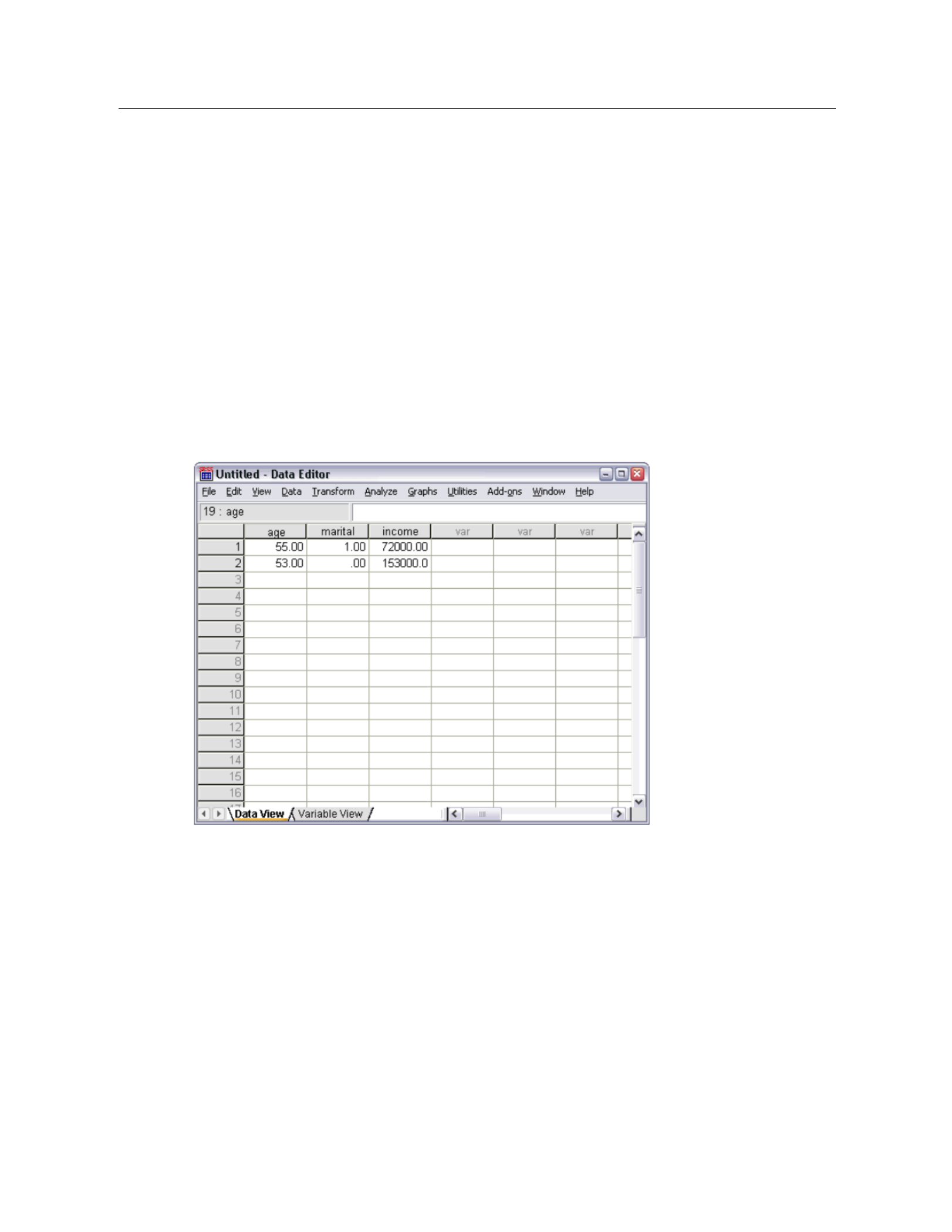
The names that you entered in Variable View are now the headings for the first three columns in
Data View.
Begin entering data in the first row, starting at the first column.
Figure 3-2
Values entered in Data View
EIn the age column, type 55.
EIn the marital column, type 1.
EIn the income column, type 72000.
EMove the cursor to the second row of the first column to add the next subject’s data.
EIn the age column, type 53.
EIn the marital column, type 0.
EIn the income column, type 153000.

28
Chapter 3
Currently, the age and marital columns display decimal points, even though their values are
intended to be integers. To hide the decimal points in these variables:
EClick the Variable View tab at the bottom of the Data Editor window.
EIn the Decimals column of the age row, type 0to hide the decimal.
EIn the Decimals column of the marital row, type 0to hide the decimal.
Figure 3-3
Updated decimal property for age and marital
Entering String Data
Non-numeric data, such as strings of text, can also be entered into the Data Editor.
EClick the Variable View tab at the bottom of the Data Editor window.
EIn the first cell of the first empty row, type sex for the variable name.
EClick the Type cell next to your entry.

29
Using the Data Editor
EClick the button on the right side of the Type cell to open the Variable Type dialog box.
Figure 3-4
Button shown in Type cell for sex
ESelect String to specify the variable type.
EClick OK to save your selection and return to the Data Editor.
Figure 3-5
Variable Type dialog box

30
Chapter 3
Defining Data
In addition to defining data types, you can also define descriptive variable labels and value labels
for variable names and data values. These d escriptive labels are used in statistical reports and
charts.
Adding Variable Labels
Labels are meant to provide descriptions of variables. These descriptions are often longer versions
of variable names. Labels can be up to 255 b ytes. These labels are used in your output to identify
the different variables.
EClick the Variable View tab at the bottom of the Data Editor window.
EIn the Label column of the age row, type Respondent's Age.
EIn the Label column of the marital row, type Mar ital Status.
EIn the Label column of the income row, type Household Income.
EIn the Label column of the sex row, type Gender.
Figure 3-6
Variable labels entered in Variable View

31
Using the Data Editor
Changing Variable Type and Format
The Type column displays the current data type for each variable. The most common data types
are numeric and string, but many other formats are supported. In the current data file, the income
variable is defined as a numeric type.
EClick the Type cell for the income row, and then click the button on the right side of the cell to
open the Variable Type dialog box.
ESelect Dollar.
Figure 3-7
Variable Type dialog box
The formatting options for the currently selected data type are displayed.
EFor the format of the currency in this example, select $###,###,###.
EClick OK to save your changes.
Adding Value L abels for Numeric Variables
Value labels provide a method for mapping your variable values to a string label. In this example,
there are two acceptable values for the marital variable. A value of 0 means that t he subject is
single, and a value of 1 means that he or she is married.
EClick the Values cell for the marital row, and then click the button on the right side of the cell to
open the Value Labels dialog box.
The value is the actual numeric value.
The value label is the string label that is applied to the specified numeric value.
EType 0in the Value field.
EType Single in the Label field.

33
Using the Data Editor
If the Value Labels menu item is already active (with a check mark next to it), choosing Value
Labels again will turn off the display of value labels.
Figure 3-9
Value labels displayed in Data View
Adding Value Labels for String Variables
String variables may require value labels as well. For example, your data may use single letters,
M For , to identify the sex of the subject. Val ue labels can be u sed to specify that Mstands
for Male and stands forF Female.
EClick the Variable View tab at the bottom of the Data Editor window.
EClick the Values cell in the sex row, and then click the button on the right side of the cell to
open the Value Labels dialog box.
EType Fin the Value field, and then type Female in the Label field.

34
Chapter 3
EClick Add to add this label to your data file.
Figure 3-10
Value Labels dialog box
EType Min the Value field, and type Male in the Label field.
EClick Add, and then click OK to save your changes and return to the Data Editor.
Because st ring v alues are case sensitive, you sh ould be consistent. A lowercase mis not the
same as an uppercase M.
Using Value Labels for Data Entry
You can use value labels for data entry.
EClick the Data View tab at the bottom of the Data Editor window.
EIn the first row, select the cell for sex.
EClick the button on the right side of the cell, and then choose Male from the drop-down list.
EIn the second row, select the cell for sex.

36
Chapter 3
Figure 3-12
Missing values displayed as periods
The reason a value is missing may be important to your analysis. For example, you may find it
useful to distinguish between those respondents who refused to answer a question and those
respondents who didn’t answer a question because it was not applicable.
Missing Values for a Numeric Variable
EClick the Variable View tab at the bottom of the Data Editor window.
EClick the Missing cell in the age row, and then click the button on the right side of the cell to
open the Missing Values dialog box.
In this dialog box, you can specify up to three distinct missing values, or you can specify a range
of values plus one additional discrete value.
Figure 3-13
Missing Values dialog box

37
Using the Data Editor
ESelect Discrete missing values.
EType 999 in the first text box and leave the other two text boxes empty.
EClick OK to save your changes and return to the Data Editor.
Now that the missing data value has been added, a label can be applied to that value.
EClick the Values cell in the age row, and then click the button on the right side of the cell to
open the Value Labels dialog box.
EType 999 in the Value field.
EType No Response in the Label field.
Figure 3-14
Value Labels dialog box
EClick Add to add this label to your data file.
EClick OK to save your changes and return to the Data Editor.
Missing Values for a String Variable
Missing values for string variables are handled similarly to the missing values for numeric
variables. However, unlike numeric variables, empty fields in string variables are not designated
as system-missing. Rather, they are interpreted as an empty string.
EClick the Variable View tab at the bottom of the Data Editor window.
EClick the Missing cell in the sex row, and then click the button on the right side of the cell to
open the Missing Values dialog box.
ESelect Discrete missing values.
EType NR in the first text box.
Missing values for string variables are case sensitive. So, a value of nr is not treated as a missing
value.

38
Chapter 3
EClick OK to save your changes and return to the Data Editor.
Now you can add a label for the missing value.
EClick the Values cell in the sex row, and then click the button on the right side of the cell to
open the Value Labels dialog box.
EType NR in the Value field.
EType No Response in the Label field.
Figure 3-15
Value Labels dialog box
EClick Add to add this label to your project.
EClick OK to save your changes and return to the Data Editor.
Copying and Pasting Variable Attributes
After you’ve defined variable attributes for a variable, you can copy these attributes and apply
them to other variables.

39
Using the Data Editor
EIn Variable View, type agewed in the first cell of the first empty row.
Figure 3-16
agewed variable in Variable View
EIn the Label column, type Age Married.
EClick the Values cell in the age row.
EFrom the menus choose:
Edit > Copy
EClick the Values cell in the agewed row.
EFrom the menus choose:
Edit > Paste
The defined values from the age variable are now applied to the agewed variable.

40
Chapter 3
To apply the attribute to multiple variables, simply select multiple target cells (click and drag
down the column).
Figure 3-17
Multiple cells selected
When you paste the attribute, it is applied to all of the selected cells.
New variables are automatically created if you paste the values into empty rows.

42
Chapter 3
All attributes of the marital variable are applied to the new variable.
Figure 3-19
All values pasted into a row
Defining Variable Properties for Categorical Variables
For categorical (nominal, ordinal) data, you can use Define Variable Properties to define value
labels and other variable properties. The Define Variable Properties process:
Scans t he actual data values and lists all unique data values for each selected variable.
Identif ies unlabeled values and provides an “auto-label” feature.
Provide s the ability to copy defined value labels from another variable to the selected variable
or from the selected variable to additional variables.
This example uses the data file demo.sav. For more information, see the topic Sample Files in
Appendix A on p. 147. This data file already has defined value labels, so we will enter a value for
which there is no defined value label.
EIn Data View of the Data Editor, click the first data cell for the variable ownpc (you may have to
scroll to the right), and then enter 99.
EFrom the menus choose:
Data > Def ine Variable Properties...

43
Using the Data Editor
Figure 3-20
Initial Define Variable Properties dialog box
In the initial Define Variable Properties dialog box, you select the nominal or ordinal variables for
which you want to define value labels and/or o ther properties.
EDrag and drop Owns TV [owntv] through Owns fax machine [ownfax] into the Variables to
Scan list.
You might notice that the measurement level icons for all of the selected variables indicate that
they are scale variables, not categorical variables. All of the selected variables in this example
are really categorical variables that use the numeric values 0 and 1 to stand for No and Yes,
respectively—and one of the variable properties that we’ll change with Define Variable Properties
is the measurement level.
EClick Continue.
44
Chapter 3
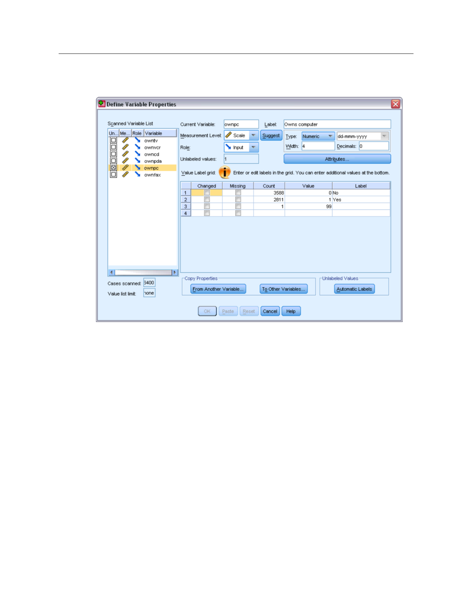
Figure 3-21
Define Variable Properties main dialog box
EIn the S canned Variable List, select ownpc.
The current level o f measurement for the selected variable is scale. You can change the
measurement level by selecting a level from the drop-down list, or you can let Define Variable
Properties suggest a measurement level.
EClick Suggest .
The Suggest Measurement Level dialog box is displayed.

45
Using the Data Editor
Figure 3-22
Suggest Measurement Level dialog box
Because the variable doesn’t have very many different values and all of the scanned cases contain
integer values, the proper measurement level is probably ordinal or nominal.
ESelect Ordinal, and then click Continue.
The measurement level for the selected variable is now ordinal.
The Value Label grid displays all of the unique data values for the selected variable, any defined
value labels for these values, and the number of times (count) that each value occurs in the
scanned cases.
The value that we entered in Data View, 99, is displayed in the grid. The count is only 1 because
we changed the value for only one case, and the Label column is empty because we haven’t
defined a value label for 99 yet. An Xin the first column of the Scanned Variable List also
indicates that the selected variable has at least one observed value without a defined value label.
EIn the Label column for the value of 99, enter No answer.
ECheck the box in the Missing column for the value 99 to identify the value 99 as user-missing.
Data values that are specified as user-missing are flagged for special treatment and are excluded
from most calculations.

47
Using the Data Editor
Figure 3-24
Apply Labels and Level dialog box
EIn the Apply Labels and Level dialog box, select all of the variables in the list, and then click Copy.
If you select any other variable in the Scanned Variable List of the Define Variable Properties
main dialog box now, you’ll see that they are all ordinal variables, with a value of 99 defined as
user-missing and a value label of No answer.
Figure 3-25
New variable properties defined for ownfax

Chapter
4
4
4
44
Working with Multiple Data Sources
Starting with version 14.0, multiple data sources can be open at the same time, making it easier to:
Switch back and forth between data sources.
Compare the contents of different data sources.
Copy and paste data between data sources.
Create multiple subsets of cases and/or variables for analysis.
Merge multiple data sources from various data formats (for example, spreadsheet, database,
text data) without saving each data source first.
Basic Handling of Multiple Data Sources
Figure 4-1
Two data sources open at same time
By default, each data source that you open is displayed in a new Data Editor window.
Any previously open data sources remain open and available for further use.
When you first open a data source, it automatically becomes the active dataset.
You can change the active dataset simply by clicking anywhere in the Data Editor window
of the data source that you want to use or by selecting the Data Editor window for that data
source from the Window menu.
© Copyright IBM Corporation 1989, 2011. 49
51
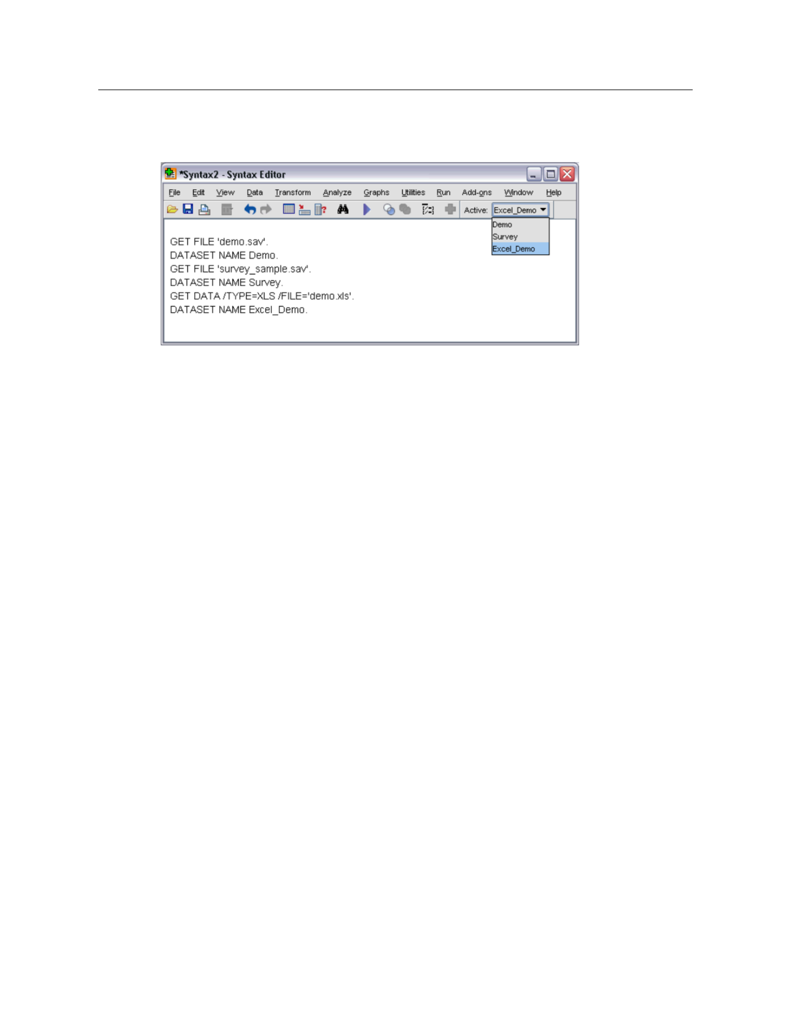
Working with Multiple Data Sources
Figure 4-3
Open datasets displayed on syntax window toolbar
Copying and Pasting Information between Datasets
You can copy both data and variable definition attributes from one dataset to another dataset in
basically the same way that you copy and paste information within a single data file.
Copying and pasting selected data cells in Data View pastes only the data values, with
no variable definition attributes.
Copying and pasting an entire variable in Data View by selecting the variable name at the top
of the column pastes all of the data and all of the variable definition attributes for that variable.
Copying and pasting variable definition attributes or entire variables in Variable View pastes
the selected attributes (or the entire variable definition) but does not paste any data values.
Renaming Datasets
When you open a data source through the menus and dialog boxes, each data source is
automatically assigned a dataset name of DataSetn, where n is a sequential i nteger value, and
when you open a data source using command syntax, no dataset name is assigned unless you
explicitly specify one with DATASET NAME. To provide more descriptive dataset names:
EFrom the menus in the Data Editor window for the dataset whose name you want to change choose:
File > Rename Dataset...
EEnter a new dataset name that conforms to variable naming rules.
Suppressing Multiple Datasets
If you prefer to have only one dataset available at a time and want to suppress the multiple
dataset feature:
EFrom the menus choose:
Edit > Options...
Termékspecifikációk
| Márka: | Ibm |
| Kategória: | Irodai szoftverek |
| Modell: | SPSS 20 |
Szüksége van segítségre?
Ha segítségre van szüksége Ibm SPSS 20, tegyen fel kérdést alább, és más felhasználók válaszolnak Önnek
Útmutatók Irodai szoftverek Ibm

8 Augusztus 2024
7 Augusztus 2024
6 Augusztus 2024
4 Augusztus 2024
Útmutatók Irodai szoftverek
Legújabb útmutatók Irodai szoftverek

1 Szeptember 2024
1 Szeptember 2024
5 Augusztus 2024
3 Augusztus 2024
29 Július 2024
27 Július 2024
26 Július 2024
26 Július 2024
25 Július 2024
20 Július 2024